posted by Lexing Xie
This post is the first of a series on modeling social media popularity using the Hawkes Intensity Process. “Expecting to be HIP (II)” gives an overview of results and interpretations on a large YouTube video dataset. “Expecting to be HIP (III)” further quantifies the effects and interpretations of promotion.
This first episode contain a rather technical overview to a new method for computing expected event rate in unit time for point processes. Understanding this is not a prerequisite for reading the subsequent posts. Such a technique is used for estimating interval-censored Hawkes processes – or when the volume of events, and not individual event times are known.
What is this about
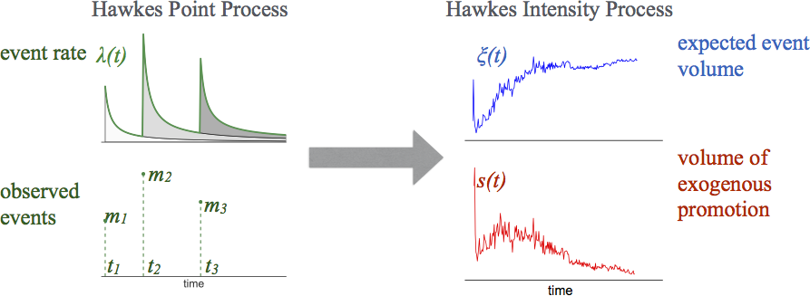
Hawkes process (Hawkes1971) is a broad-class of stochastic processes when seeing an event (something happens at a given time) increases likelihood of seeing other events shortly after that. It has been widely used in problems from earth quake modeling, finance, criminology, and most recently, in modeling behavior and attention in social media.
Hawkes process decribes the probability of seeing a new event given all previous events. Here $\mu$ is a scaling parameter, $s(t)$ is external stimuli, and $\phi(\tau)$ is a kernel function over time that describe the influence of a past event to future events. $$\lambda(t) = \mu s(t) + \sum_{t_i < t} \phi(t-t_i) $$
In many real-world scenarios, we observe the volume of activities, but do not observe individual activities itself. Think, for example, Google Trends for comparing search volume, or the web traffic logs. We call this quantiy expected event volume, or $\xi(t)$. It is somewhat surprising, that we found no analytical expression for $\xi(t)$ in the literature.
How is this done?
Here we take the opposite approach to the paper, by explaining the rationale behind the derivation backwards, in the hope that this complements the paper content and gives insight about how we arrived at the particular form. The end result of computing such an expectation is an analytical expression that relates $\xi(t)$ to its own history $\xi(t-\tau)$ at offset $\tau$ discounted by memory kernel $\phi(\tau)$.
$$\xi(t) = \mu s(t) + \int_0^t \xi(t-\tau) \phi(\tau) d\tau $$
Here are a few key steps for arriving at this integral equation. Although somewhat technical, they are individually easy in the sense that it does not require formal mathematical knowledge beyond probability and calculus.
- Precisely define what the expectation is taken over. In this case, it is over the random function $N(t)$ (called the counting process), that represent the number of event happened so far at any given time $t$. Note that the piece-wise constant random function $N(t)$ is equivalent to event history $\cal H$, containing all time stamps of the random number of events happened before time $t$.
- Notice that $\mu s(t)$ is non-random, therefore it does not change after expectation.
- Notice that a key difference between $\lambda(t)$ and $\xi(t)$ is to go from a summation of individual events, to an integration in continuous time. Remember from calculus 101 that an integration can be seen as summing over infinitesimal intevals, with the size of interval approaches zero $\delta\downarrow 0$.
- Realize that taking expecations over $N(t)$ is equivalent to taking expectations over its increments $dNt$ computed over small intervals of size $\delta$. These increments are binary (0 or 1) – therefore converting a hard problem of avearging over random non-smooth function $N(t)$ into a set of binary Bernouli variables.
- Recall from any point process textbook, that the event rate $\lambda(t)$ can be defined as the probability of seeing one event in a small interval $\delta$ times the size of the interval. Therefore the expectation of binary Bernouli variables is nothing but $\delta\lambda(t)$.
- We are nearly there! Exchange the order of expectation and limit, take care of the indices of intervals $\delta$, and apply the definition of $\xi(t)$ yields the convolution form above.
Writing out the above formally, you will prove the expression about $\xi(t)$ above, as shown in Equation (4)-(11) from the supplemental section of the preprint. This is not hard to extend to marked point processes, where the expectation is also over independently drawn set of event magnitudes.
Looking through the literature, (Hawkes1971) computes the covariance density of the point-process but not expected event rate, and (Helmstetter2002) mentions a Wiener-Hopf integram equation, but the precise meaning and derivation was omitted from the manuscript. If you know Martingale theory, then you may be interested in this alternative proof provided by Young Lee at Data61.
Broader implications
One may think that this is a rather dry result. However this allows a series of analysis and model estimation to be done on volume, instead of instance, data. This brings huge advantages in terms of computational cost (think: millions of instances versus hundreds of days), it also faciliates scenarios where data access is limited, and protects privacy. For exmaple:
- Social behavior of the masses – the volume of activities in something (a video, a website, a search term) is often much easier to obtain and do computation on than the individual events. One critical advantage in being able to compute over volumes is to be able to link different sources of information. One could ask questions like: how much does google search drive traffic in these NYTimes pages, Wiki pages, the corresponding YouTube video?
- Epidemiology – it can be easy (for people outside of the medical profession and CDC) to collect the volume of a disease (e.g. flu) rather than individual instances due to strict privacy concerns. Again, it is the linking of real-world quantities such as aggregate sales to health outcomes that should enable us to make novel observations and draw interesting conclusions.
- Finance and stock trading – The algorithmic trading community are already struggling with high volumes of transactions. There is promise for uncovering global market trends with much less computation, if we are able to compute on trading volume in time, rather than individual transactions generated by thousands or millions of machines.
Using the HIP model, we obtained several fun observations about YouTube videos, including which videos cannot be promoted, or which ones are likely to be viral but have not done so. Details of these observations can be found in the “Expecting to be HIP (II)” post, or – read the paper : )
On the more technical end, we also hope the method outlined above will come in handy for similar results involving the relationship between individual events in time and expected volumes, such as for epidemic models. On the other hand, we can also hope to generalize this method to moment-matching methods for estimating interval-censored Hawkes processes, this is forthcoming with Young Lee and Kar Wai Lim at Data61.
Resources
Marian-Andrei Rizoiu, Lexing Xie, Scott Sanner, Manuel Cebrian, Honglin Yu and Pascal Van Hentenryck. Expecting to be HIP: Hawkes Intensity Processes for Social Media Popularity, in Proceedings International Conference on World Wide Web (WWW ‘17), Perth, Australia, 2017.
| Download: | Paper PDF + SI Talk slides |
| Data: | ACTIVE Dataset and source code Interactive visualization system |
| Bibtex: |
@inproceedings{Rizoiu2017,
    address = {Perth, Australia},
    author = {Rizoiu, Marian-Andrei and Xie, Lexing and Sanner, Scott and Cebrian, Manuel and Yu, Honglin and {Van Hentenryck}, Pascal},
    booktitle = {World Wide Web 2017, International Conference on},
    pages = {1--9},
    title = {{Expecting to be HIP: Hawkes Intensity Processes for Social Media Popularity}},
    year = {2017}
}
References
- Hawkes, A.G.: Spectra of some self-exciting and mutually exciting point processes. Biometrika 58(1), 83–90 (Apr 1971)
- Helmstetter, A., Sornette, D.: Subcritical and supercritical regimes in epidemic models of earthquake aftershocks. Journal of Geophysical Research: Solid Earth 107(B10), ESE 10–1–ESE 10–21 (2002)